Modelling Programming Languages
Contents
- Overview
- Lambda-Calculus
- Displaying the Calculus
- Type Checking the Calculus
- Evaluation by Machine
- Extending the Machine
Overview
There are many different types of model used to analyse programs and programming languages. These include models of source code, e.g. flow-graphs, models of type systems, models of pre and post conditions, petri-nets and various calculi.Models of programs and their languages are important because designing and implementing programs, as anyone knows who has tried it for real, is a challenging task. The key features of what makes a program work, are hidden away inside a black-box. Even if it was possible to look inside the box, all that would be revealed is a bunch of electronics, memory addresses, registers and binary data.
Programs are not designed in terms of the implementation platform that is eventually used to run the code. A program is defined and implemented in terms of models that describe various abstractions over the implementation platform. The models make programming feasible for humans.
A key model that is used when constructing programs, is the programming language itself. When the code is eventually performed on the machine, the program that was written by the human engineer is certainly not executed directly by the hardware. Over time, languages have been developed that provide abstractions over the implementation platform.
Having said that current programming languages (their libraries and the various software platforms that are currently used) are abstractions; they still must deal with many features of implementation detail that allow the hardware to poke through. Take any serious programming language manual and there will be a section describing how to make the thing run as fast as possible. Use any commercial library (graphics libraries being a case in point) and there will be many features that, whilst they shield the user from the basic underlying hardware, still seem fairly complex.
There is a grand history of models of programming languages. These models are used to understand the fundamentals of what essential features make a program work for an intended application. If you like, these models are an abstraction of an abstraction, but don't let that put you off; a familiarity with these models is a sure step in the direction of being in-control of a wide range of programming notations.
One of the most important programming language models is the lambda-calculus. It is essentialy a model of procedure-call (and method-call) based languages and has be used to model languages including Pascal, Ada, and Java. There are plenty of texts describing the lambda-calculus and it is certainly not the intent of this book to provide a tutorial. Many of the texts are quite theoretical in nature and should be ignored; pick out some of the more practical looking texts if you are interested, it is certainly worth it.
The rest of this section shows how the lambda-calculus can be modelled. In particular, a machine is developed that runs the calculus. The SECD machine is a fantastic tool to understand how programming languages tick. It is simple and can be extended in a miriad of ways to model useful abstractions of programming language execution.
To top.
Lambda-Calculus
The syntax of the lambda-calculus is defined as follows:E ::= ExpressionsWhere an expression is either a variable (just a name), a function (1 arg and an expression body) or an application (of a function to an arg).
V Variables
| \V.E Functions (of 1 arg)
| E E Applications
The execution of any calculus expression is also quite simple and takes place with respect to an environment that associates variable names with values. To evaluate a variable, look up the variable name in the environment. To evaluate a function, produce a closure that associates the function with the current environment. To evaluate an application, first evaluate the function and arg expressions to produce a closure and a value. Evaluate the body of the closure-function with respect to the closure-environment extended by associating the closure-arg with the arg-value.
The execution is the essence of programming language execution where procedure (method) calls evaluate by supplying the arguments and then wherever the body of the procedure refers to the argument by name, the supplied value is used instead. Of course there are many caveats and special cases (not least order of evaluation and side-effects), but these can all be dealt with by equipping the basic calculus with the right machinery. The basic calculus is modelled as follows:
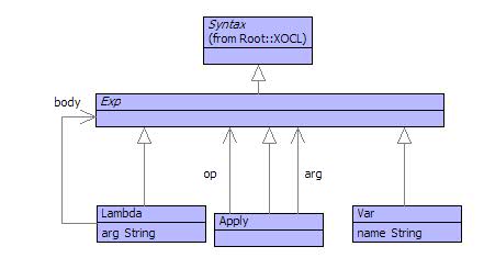
The class Exp extends Syntax so that lambda expressions are self-evaluating. The grammar is as follows:
@GrammarThe definition of Composite provides an interesting feature: left association. Applications are left associative in the lambda-calculus, therefore the expression a b c is grouped as the application a b applied to c, or equivalently (a b) c. The Composite rule is defined using an argument a that accumulates the applications to the left.
Exp ::=
Exp1 'end'.
Exp1 ::=
Lambda
| a = Atom Composite^(a).
Lambda ::=
'\' a = Name '.' e = Exp1
{ Lambda(a,e) }.
Composite(a) ::=
b = Atom c = { Apply(a,b) } Composite^(c)
| b = Lambda { Apply(a,b) }
| { a }.
Atom ::=
Var
| Integer
| '(' Exp1 ')'.
Var ::=
n = Name { Var(n) }.
end
To top.
Displaying the Calculus
The basic output mechanisms supported by XMF will display expressions in the calculus in a general purpose format. Howeever, it would be nicer if the abstract syntax expressions could be displayed in a form that was the same as the concrete syntax.A naive implementation just translates each expression back into the string that corresponds to the concrete syntax. However, this will produce errors since the original expressions may have been grouped using parentheses. For example, the expression N M O wil be read as (N M) O and not N (M O). The display operation muct be implemented to finsert parentheses when required in order to allow the rendered output to be read back in.
To do this we invent a notion of precedence. Each expression has a precedence level at which it can be displayed. If the current precedence level is equal to or greater than the expression's designated precedence then no parentehses are required. Otherwise, the expression must be protected using parentheses. The precedence levels are defined as global bindings in the definition of the Calculus package:
context SECDThe EXP_PREC is the highest level where no protection is required. For the simple calculus only a lambda-expression and an application needs to be protected so these have their own precedence levels.
@Package Calculus
@Bind EXP_PREC = 2 end
@Bind LAMBDA_PREC = 1 end
@Bind APPLY_PREC = 0 end
end
Next, we implement a general purpose display operation. All syntax implements a pprint() operation that returns a string. So if this is implemented for Exp then this will hook-in to the XMF syntax display mechanisms:
import Calculus;Now we must implement a pprint1 operation for each of the syntax classes:
context Exp
@AbstractOp pprint1(opPrec:Integer):String
end
context Exp
@Operation pprint():String
self.pprint1(EXP_PREC)
end
context ApplyTo top.
@Operation pprint1(opPrec:Integer):String
if opPrec < APPLY_PREC
then "(" + op.pprint1(opPrec) + " " + arg.pprint1(opPrec) + ")"
else op.pprint1(APPLY_PREC - 1) + " " + arg.pprint1(APPLY_PREC)
end
end
context Lambda
@Operation pprint1(opPrec:Integer):String
if opPrec < LAMBDA_PREC
then "(" + "\\" + arg + "." + body.pprint1(EXP_PREC) + ")"
else "\\" + arg + "." + body.pprint1(LAMBDA_PREC)
end
end
context Var
@Operation pprint1(opPrec)
name
end
Type Checking the Calculus
Not all expressions in the lambda-calculus are legal in the sense that they cannot be executed. If we view lambda as a (very simple) programming language then the illegal expressions would either not get through the compiler or would cause the program to abort at run-time.A key check for legal expressions is type correctness. Execution involves performing operations on data items. An expression is type correct no operation gets a surprise: only legal data items are supplied to operations.
Some languages are statically typed which means that type correctness can be established before a program in the language is performed. Lambda is an example of a statically typed language. Furthermore, if an expression in the lambda-calculus is correctly typed then there are rules that can deduce the type without the need for the types to be inserted into the expressions.
Although it is rare for programming languages to have statically deduced types, it is useful to know how this works in order to have a flexible model of a program execution from start to finish. This section shows how simple types can be modelled in XMF for the lambda-calculus and how XRules can be used to implement the deduction rules for the calculus.
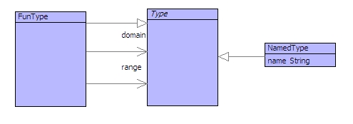
Each expression has a type which is either a function type or a named type:
The rules for the calculus are defines in an XRules rule-base which is created as follows:
parserImport XOCL;The rule-base defined a single rule named Type which associates three things:
parserImport XRules;
import XRules;
import SECD;
import Calculus;
import Types;
context SECD
@Rules Check import Root, Calculus, Types
// The rules will be added to the Check rule-base.
// The rule-base must import the packages containing
// classes that the rules will reference.
end
- An environment associating variable names with their types.
- An expression.
- A type.
context CheckThe clause defined above is a relationship between three elements. If the first element is a sequence of the given format, the second is a variable whose name occurs as the head of the first binding in the sequence and the third element is the tail of the first binding in the sequence then the clause is satisfied.
@Rule Type(Seq{Seq{Name | Type} | Rest},
Var[name=Name],
Type)
end
Optionally, a clause may have a body which lists further conditions on the supplied elements. In this case, the body of the clause is empty.
The clause defined above defines the case where we are type-checking a variable and the variable is the first entry in the environment of variables and types. In this case you can think of the clause as returning the type at the head of the environment (but really we should think of the clauses as defining a relation between all the arguments).
What happens when the name is not the first entry in the environment? The clause defined above will fail to be satisfied, so we need another clause:
context CheckIn this case the clause has a body that states that the type associated with the supplied variable can be found in the rest of the environment. The two clauses defines so far overlap: given any three elements, sometimes the first clause will be satisfied, often both will be satisfied and sometimes neither clause will be satisfied. When clauses overlap, order is important in XRules. The first clause to be satisfied is chosen, and in this case the order is that as given above.
@Rule Type(Seq{Ignore | Env},Var[name=Name],Type)
// The type of the variable called Name is Type
// with respect to the supplied environment
// Seq{Ignore | Env} when the type of the variable
// is Type in the environment Env...
Type(Env,Var[name=Name],Type)
end
An application involves an operator and an argument. An operator has a function-type which consists of a domain-type (the type of expected arguments) and a range-type (the type of results). In order for the application to be well-typed, the domain type must match the type of the argument. If it does, then the type of the application expression is the range-type:
context CheckFinally, a lambda-expression has a function-type that is constructed by extending the supplied environment with a type for the argument (the domain-type) and constructing a range-type from the body of the lambda-expression:
@Rule Type(Env,Apply[op=Operator;arg=Arg],Range)
// The the of the application is Range when
// the type of the operator is Domain -> Range
// and the type of the argument is Domain...
Type(Env,Operator,FunType[domain=Domain;range=Range])
Type(Env,Arg,Domain)
end
context CheckThat concludes the type-checking rules for a basic lambda-calculus. XRules has been used because this is a relational rule-based language (like Prolog) that allows the types of lambda-expressions to be deduced, i.e. you can supply an environment and a lambda-expression to the rule-base and it will construct a type if one exists. To do this, suppose that we have a collection of builtin operators for the calculus whose types are given by the operator typeEnv as follows:
@Rule Type(Env,Lambda[arg=Arg;body=Body],FunType[domain=Domain;range=Range])
// The type of a lambda-expression \Arg.Body is Domain -> Range with
// respect to tne environment Env when the type of Body is
// Range with respect to the extended environment:
// Seq{Seq{Arg | Domain} | Env} ...
Type(Seq{Seq{Arg | Domain} | Env},Body,Range)
end
context SECDWhen using XRules, the form @WithRules can be used to call a rule in a rule-base and to extract the value of one or more variables from the result:
@Operation typeEnv()
// Returns an environment for use as the initial
// context for type checking an expression. All the
// names defined here are in scope...
Seq{
Seq{"add1" | FunType(NamedType("Int"),NamedType("Int"))},
Seq{"isZero" | FunType(NamedType("Int"),NamedType("Bool"))},
Seq{"not" | FunType(NamedType("Bool"),NamedType("Bool"))},
Seq{"zero" | NamedType("Int")}
}
end
parserImport XRules;The above expression produces:
import XRules;
@WithRules(Check)
// Call the following rule...
Type(<typeEnv()>,Apply[op=Var[name="add1"];arg=Var[name="zero"]],T)
// Return the value of the following variable...
return T
end
NamedType(Int)
A slightly more complex expression involves two applications. Note that
the return type of the add1 operation must match the argument type of
the isBool operation:@WithRules(Check)produces:
Type(<typeEnv()>,Apply[op=Var[name="isZero"];arg=Apply[op=Var[name="add1"];arg=Var[name="zero"]]],T)
return T
end
NamedType(Bool)
Finally, to show what happens when an expression has no type, consider
the following:@WithRules(Check)where the return type of isBool does not match the expected argument type of add1. In this case no type can be deduced for the expression and the return value is:
Type(<typeEnv()>,Apply[op=Var[name="add1"];arg=Apply[op=Var[name="isZero"];arg=Var[name="zero"]]],T)
return T
end
FAIL
To top.
Evaluation by Machine
Execution of lambda-calculus expressions can be performed by the SECD
machine whose states are shown below: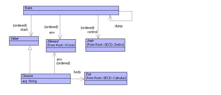
The machine is referred to as the SECD-machine because it has 4 components:
- The stack S that is used to hold intermediate results from expressions.
- The environment E that is used to associate variable names with values.
- The control C that is used to hold sequences of machine instructions.
- The dump D that is used to hold resumptions.
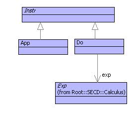
Any expression is translated into an instruction using Do. The App instruction is used to perform an application as shown below. The best way to see what how the SECD machine works is to see it running. The following trace shows the execution of an expression (\v. v v)(\x.x). In order to make the output readable, the following pretty-printers have been defined for the various classes:
- States: (s,e,c,d)
- sequences: [x1,x2,x3]
- pairs: h->t
- App: @
- Do: ignored.
(1) ([],[],[(\v.v v) (\x.x)],null)The first thing to appreciate about the evaluation is roughly what the expression is doing: the function \v.v v is aplied to the function \x.x causing the function \x.x to be applied to itself producing the result \x.x. Now look at the trace and step through it to see how a machine evaluates the expression. Each step in the trace is a new machine state produced from the previous state by performing a transition. A transition looks at the head of the control in the pre-state to determine the next state.
(2) ([],[],[(\x.x),(\v.v v),@],null)
(3) ([<x,[],x>],[],[(\v.v v),@],null)
(4) ([<v,[],v v>,<x,[],x>],[],[@],null)
(5) ([],[v-><x,[],x>],[v v],([],[],[],null))
(6) ([],[v-><x,[],x>],[v,v,@],([],[],[],null))
(7) ([<x,[],x>],[v-><x,[],x>],[v,@],([],[],[],null))
(8) ([<x,[],x>,<x,[],x>],[v-><x,[],x>],[@],([],[],[],null))
(9) ([],[x-><x,[],x>],[x],
([],[v-><x,[],x>],[],
([],[],[],null)))
(10) ([<x,[],x>],[x-><x,[],x>],[],
([],[v-><x,[],x>],[],
([],[],[],null)))
(11) ([<x,[],x>],[v-><x,[],x>],[],([],[],[],null))
(12)([<x,[],x>],[],[],null)
Line (1) is the initial state. the expression is loaded onto the control. Everything else is empty. Transition (1-2) performs the application expression by unpacking it at the head of the control and adding an @ instruction. Transition (2-3) evaluates the function \x.x to produce the closure at the head of the stack. Notice how the stack is used to hold intermediate results; machine transitions consume 0 or more values at the head of the stack and produce 0 or 1 new values at the head of the stack. Transition (3-4) evaluates the function \v. v v. Transition (4-5) performs the @ instruction by setting up the evaluation of the body of the operator. The state of the machine is saved in the dump so that the return value from the application can be used. Notice how the envirnment in the new state (5) contains a binding for the arg v. Transition (5-6) evaluates the application v v. Transitions (6-9) evaluate the two references to the variable v and then perform the application (again saving the current state for return). Transition (9-10) evaluates the reference to x and (10-11) returns a value since the control is exhausted. Transition (11-12) perfoms the final return leaving the value of the original expression at the head of the stack.
The rules of evaluation for the basic lambda-calculus are very simple. They can be described using pattern matching and are defined in the operation trans below that performs a single transition. A good understanding of the rules of evaluation and their many variations is an excellent basis for a deep understanding of how modelling can inform and enrich programming.
@Operation trans(state:State):StateTransition (1) evaluates a variable by looking its name up in the current environment and pushing the value on the stack. Transition (2) unpacks an application at the head of the control. Transition (3) performs an @ instruction at the head of the control. It expects a closure above an argument at the head of the stack. The current state is pushed onto the dump and a new state is created from the closure body and environment. Transition (4) defines evaluation of a function. Finally, transition (5) describes how a value is returned from a completed function application (the body is exhausted).
@Case state of
(1) State(s,e,Seq{Do(Var(n))|c},d) do
State(Seq{e.lookup(n)|s},e,c,d)
end
(2) State(s,e,Seq{Do(Apply(o,a))|c},d) do
State(s,e,Seq{Do(a),Do(o)} + Seq{App()|c},d)
end
(3) State(Seq{Closure(n,e1,b),a} + s,e2,Seq{App()|c},d) do
State(Seq{},e1.bind(n,a),Seq{Do(b)},State(s,e2,c,d))
end
(4) State(s,e,Seq{Do(Lambda(n,b))|c},d) do
State(Seq{Closure(n,e,b)|s},e,c,d)
end
(5) State(Seq{v},e1,Seq{},State(s,e2,c,d)) do
State(Seq{v|s},e2,c,d)
end
end
end
To top.
Extending the Machine
As it stands, the calculus and its execution by the SECD machine does
not look much like a standard programming language. Using just the
features you have seen, it is possible to encode virtually all standard
programming language concepts. Doing so is a bit like a cryptic
crossword - fiendishly difficult and spectacularly rewarding.Rather than work with models of programs at the basic calculus level, it is usual to add extensions. In fact, this is where the calculus and its mechanical execution starts to be useful: if you have a requirement to understand or design a new novel feature then see what you need to do to add it to the calculus and SECD machine.
This section shows how the basic model can be extended by adding records, integers and builtin operations such as +. A record is represented as in [age=56, yearsService=10]. A tuple, or vector, is a record where the fields have pre-determined names (usually represented as numbers); for example a pair is [fst=1,snd=2] rather than (1,2). This allows builtin operations to take tuples (represented as records) as arguments: add[fst=1,snd=2] is the same as 1 + 2.
The extensions to the syntax model are shown below:

The grammar is modified as follows:
Atom ::=The following shows an execution of the expression (\x.\y.add[fst=x,snd=y]) 10 20. The builtin environment is shown as E. E contains a binding for the name add to the builtin operation for +.
Var
| Record
| Integer
| '(' Exp1 ')'.
Record ::=
'[' f = Field
fs = (',' Field)*
']'
{ Record(Seq{f|fs}) }.
Field ::=
n = Name
'=' e = Exp1
{ Field(n,e) }.
Integer ::=
i = Int
{ Integer(i) }.
([],E,[(\x.\y.add [fst=x,snd=y]) 10 20],null)There are a number of ways of handling builtin operations. The following shows how the add operation is builtin to the transitions performed by the machine:
([],E,[20,(\x.\y.add [fst=x,snd=y]) 10,@],null)
([20],E,[(\x.\y.add [fst=x,snd=y]) 10,@],null)
([20],E,[10,(\x.\y.add [fst=x,snd=y]),@,@],null)
([10,20],E,[(\x.\y.add [fst=x,snd=y]),@,@],null)
([10,20],E,[\x.\y.add [fst=x,snd=y],@,@],null)
([<x,E,\y.add [fst=x,snd=y]>,10,20],E,[@,@],null)
([],E[x->10],[\y.add [fst=x,snd=y]],
([20],E,[@],null))
([<y,E[x->10],add [fst=x,snd=y]>],E[x->10],[],
([20],E,[@],null))
([<y,E[x->10],add [fst=x,snd=y]>,20],E,[@],null)
([],E[y->20,x->10],[add [fst=x,snd=y]],([],E,[],null))
([],E[y->20,x->10],[[fst=x,snd=y],add,@],([],E,[],null))
([],E[y->20,x->10],[x,y,{fst,snd},add,@],([],E,[],null))
([10],E[y->20,x->10],[y,{fst,snd},add,@],([],E,[],null))
([20,10],E[y->20,x->10],[{fst,snd},add,@],([],E,[],null))
([[fst=10,snd=20]],E[y->20,x->10],[add,@],([],E,[],null))
([!add,[fst=10,snd=20]],E[y->20,x->10],[@],([],E,[],null))
([30],E[y->20,x->10],[],([],E,[],null))
([30],E,[],null)
@Operation trans(state:State):StateTo top.
@Case state of
State(Seq{v},e,Seq{},d) when d = null do
v
end
State(s,e,Seq{Do(Var(n))|c},d) do
State(Seq{e->lookup(n)|s},e,c,d)
end
State(s,e,Seq{Do(Apply(o,a))|c},d) do
State(s,e,Seq{Do(a),Do(o)} + Seq{App()|c},d)
end
State(s,e,Seq{Do(Paren(x))|c},d) do
State(s,e,Seq{Do(x)|c},d)
end
State(Seq{Closure(n,e1,b),a} + s,e2,Seq{App()|c},d) do
Root::indent := indent + 2;
State(Seq{},e1.bind(n,a),Seq{Do(b)},State(s,e2,c,d))
end
State(s,e,Seq{Do(Lambda(n,b))|c},d) do
State(Seq{Closure(n,e,b)|s},e,c,d)
end
State(s,e,Seq{Do(Record(fs))|c},d) do
State(s,e,fs->collect(f | Do(f.exp)) + Seq{Rec(fs.name)|c},d)
end
State(s,e,Seq{Do(Integer(i))|c},d) do
State(Seq{Const(i)|s},e,c,d)
end
State(s,e,Seq{Rec(ns)|c},d) do
State(Seq{Tuple(s->take(ns->size)->reverse->zip(ns)->collect(p | Slot(p->tail,p->head)))|s->drop(ns->size)},e,c,d)
end
State(Seq{Builtin("add"),Tuple(Seq{Slot("fst",Const(n1)),Slot("snd",Const(n2))})} + s,e,Seq{App()|c},d) do
State(Seq{Const(n1+n2)|s},e,c,d)
end
State(Seq{v},e1,Seq{},State(s,e2,c,d)) do
Root::indent := indent - 2;
State(Seq{v|s},e2,c,d)
end
end
end